Time Series in R: Quick Reference

Read and Define the Time Series (TS) Objects

---

Read from a Saved File

These functions reads a file without a TS structure and then defines the TS object.

# Read from a raw csv file
raw.data <- read.table("./data/data.us.csv", sep = ",", header = T)

# When you have the dates in the original csv file
xts.data <- xts(raw.data, order.by = as.Date(raw.data$date, "%m/%d/%Y"))

# When you don't have the dates in the original csv file but know the starting date
date = seq(as.Date("1960/3/1"), by = "3 month", length.out = nrow(raw.data))
xts.data <- xts(raw.data[,-1], order.by = date, frequency = 3)

This function reads and declares the TS structure from the begining.

# Note that this is a TS with a zoo structure
ts.data <- read.zoo("./data/data.us.csv", index.column = 1, sep = ",", header = T, format = "%m/%d/%Y")
# Or...
ts.data <- ts(raw.data[,2:4], frequency = 4, start = c(1960,1))

# One can convert the TS-zoo into a xts...
xts.data <- as.xts(ts.data)

---

Read from Online Sources

There are two main ways to get data into R: get the data into Excel or a csv or download for an online source. There are built-in package to get the data directly for the web in a predefined format. The table below shows the most popular sources and packages that one can use.

Sources	R-Package	Web Pages
Yahoo, FRED, Google, Onda	quantmod	Link
International Monetary Fund (IMF)1	IMFData or imfr	Link
World Bank’s WDI	WDI	Link
OECD2	rsdmx	Link
Penn World Tables	pwt	Link
International Labor Organization (ILO)	rsdmx	Link

One can use the getSymbols function with a previous search in the web pages and download directly into R.

getSymbols("GDPC1", src = "FRED")
getSymbols("PCEPILFE", src = "FRED")
getSymbols("FEDFUNDS", src = "FRED")

names(GDPC1) <- "US Real GDP"
names(PCEPILFE) <- "Core PCE"
names(FEDFUNDS) <- "FED Rate"

---

Subset and Extract

# Federal funds rate, montly data from January 1980 to March
FEDFUNDS["1980-01-01/1980-03-01"]

           FED Rate
1980-01-01    13.82
1980-02-01    14.13
1980-03-01    17.19

# Real GDP, quarterly data, for in 2006
GDPC1["2006"]

           US Real GDP
2006-01-01    15244.09
2006-04-01    15281.52
2006-07-01    15304.52
2006-10-01    15433.64

# End of period inflation rate from 2000 to 2005
PCEPILFE[format(index(PCEPILFE["2000/2005"]), "%m") %in% "12"]

           Core PCE
1959-12-01   17.029
1960-12-01   17.255
1961-12-01   17.458
1962-12-01   17.677
1963-12-01   17.972
1964-12-01   18.201

---

Identify ’NA’s, Fill and Splice

# Set missings into the series...
gdp.miss <- GDPC1["2000/2002"]
gdp.miss["2001"] <- NA

# Identify the NAs
gdp.miss[is.na(gdp.miss)]

# Show numbers without NAs
na.omit(gdp.miss)

# Fill missing with the last observarion or with the first non-missing
# observation
cbind(gdp.miss, na.locf(gdp.miss), na.locf(gdp.miss, fromLast = T))

           US.Real.GDP US.Real.GDP.1 US.Real.GDP.2
2000-01-01    12935.25      12935.25      12935.25
2000-04-01    13170.75      13170.75      13170.75
2000-07-01    13183.89      13183.89      13183.89
2000-10-01    13262.25      13262.25      13262.25
2001-01-01          NA      13262.25      13394.91
2001-04-01          NA      13262.25      13394.91
2001-07-01          NA      13262.25      13394.91
2001-10-01          NA      13262.25      13394.91
2002-01-01    13394.91      13394.91      13394.91
2002-04-01    13477.36      13477.36      13477.36
2002-07-01    13531.74      13531.74      13531.74
2002-10-01    13549.42      13549.42      13549.42

# Fill missing values with linear interpolation and bubic spline
cbind(gdp.miss, na.approx(gdp.miss), na.spline(gdp.miss, method = "fmm"))

           US.Real.GDP US.Real.GDP.1 US.Real.GDP.2
2000-01-01    12935.25      12935.25      12935.25
2000-04-01    13170.75      13170.75      13170.75
2000-07-01    13183.89      13183.89      13183.89
2000-10-01    13262.25      13262.25      13262.25
2001-01-01          NA      13288.96      13319.23
2001-04-01          NA      13315.08      13335.55
2001-07-01          NA      13341.50      13337.02
2001-10-01          NA      13368.20      13348.30
2002-01-01    13394.91      13394.91      13394.91
2002-04-01    13477.36      13477.36      13477.36
2002-07-01    13531.74      13531.74      13531.74
2002-10-01    13549.42      13549.42      13549.42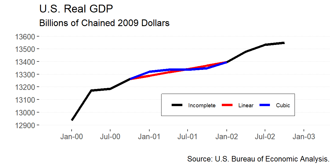

---

Transformations, Combine and Change Frequency

---

Basic Function Transformations

Transformation	Command
Logarithm	log(y)
Lag: \(L^{n} y_{t} = y_{t-1}\)	lag(y,n)
Difference: \(\Delta y_{t} = y_{t} - y_{t-1}\)	diff(y)
Moving average: \(\bar{y}^{n}_{t} = \frac{1}{n} \sum^{n-1}_{i=0} y_{t-i}\)	rollapply(y, n, FUN = mean)
Cumulative sum: \(y^{s}_{t} = \sum^{t}_{i=0} y_{i}\)	cumsum(y)

# Transformations
xts.gdp$lgdp <- log(xts.gdp$gdp)
xts.gdp$lgdp_1 <- lag(xts.gdp$lgdp, 1)
xts.gdp$dlgdp <- diff(xts.gdp$lgdp)
xts.gdp$mov.avg5_lgdp <- rollapply(xts.gdp$lgdp, 5, FUN = mean)
xts.gdp$cu.sum_lgdp <- cumsum(xts.gdp$lgdp)

---

Period aggregation

# Get a date index on a lower frequency
periodicity(xts.gdp)

Quarterly periodicity from 1947-03-01 to 2023-03-01 

years <- endpoints(xts.gdp, on = "years")

# Aggregate to first/end of period
xts.gdp.a.firs <- period.apply(xts.gdp, INDEX = years, FUN = first)
xts.gdp.a.last <- period.apply(xts.gdp, INDEX = years, FUN = last)
# Aggregate to average of period
xts.gdp.a.mean <- period.apply(xts.gdp, INDEX = years, FUN = mean)
# Aggregate to sum of period
xts.gdp.a.sum <- period.apply(xts.gdp, INDEX = years, FUN = sum)
# Aggregate to min/max of period
xts.gdp.a.min <- period.apply(xts.gdp, INDEX = years, FUN = min)
xts.gdp.a.max <- period.apply(xts.gdp, INDEX = years, FUN = max)

# Putting all together...
cbind(xts.gdp["2000/2001"], xts.gdp.a.firs["2000/2001"], xts.gdp.a.last["2000/2001"],
    xts.gdp.a.mean["2000/2001"], xts.gdp.a.sum["2000/2001"], xts.gdp.a.min["2000/2001"],
    xts.gdp.a.max["2000/2001"])

            QRT.GDP  FOP.GDP  EOP.GDP  AVG.GDP  SUM.GDP  MIN.GDP  MAX.GDP
2000-03-01 12935.25       NA       NA       NA       NA       NA       NA
2000-06-01 13170.75       NA       NA       NA       NA       NA       NA
2000-09-01 13183.89       NA       NA       NA       NA       NA       NA
2000-12-01 13262.25 12935.25 13262.25 13138.04 52552.14 12935.25 13262.25
2001-03-01 13219.25       NA       NA       NA       NA       NA       NA
2001-06-01 13301.39       NA       NA       NA       NA       NA       NA
2001-09-01 13248.14       NA       NA       NA       NA       NA       NA
2001-12-01 13284.88 13219.25 13284.88 13263.42 53053.67 13219.25 13301.39

---

Combine series

# Aggregate data to quarterly averages
quarts <- endpoints(xts.inf, on = "quarters")
xts.inf.q.avg <- period.apply(xts.inf, INDEX = quarts, FUN = mean)

# Merge monthly and quarterly data
xts.inf <- merge(xts.inf, xts.inf.q.avg, join = "left")
colnames(xts.inf) <- c("EOP.inf", "AVG.inf")
xts.inf["2001"]

           EOP.inf  AVG.inf
2001-01-01  81.592       NA
2001-02-01  81.736       NA
2001-03-01  81.821 81.71633
2001-04-01  81.951       NA
2001-05-01  81.970       NA
2001-06-01  82.154 82.02500
2001-07-01  82.366       NA
2001-08-01  82.406       NA
2001-09-01  81.939 82.23700
2001-10-01  82.516       NA
2001-11-01  82.683       NA
2001-12-01  82.702 82.63367

# Merge two series and exclude the missing cases from both sides
merge(xts.gdp["2001"], xts.inf["2001"], join = "inner")

            QRT.GDP EOP.inf  AVG.inf
2001-03-01 13219.25  81.821 81.71633
2001-06-01 13301.39  82.154 82.02500
2001-09-01 13248.14  81.939 82.23700
2001-12-01 13284.88  82.702 82.63367

---

Summary Charts

# Plot separate series under the zoo TS structure
plot(ts.data[,c(1:2)], plot.type = "multiple",
     col = c("blue","red"),
     lty = c(1,1), lwd = c(2,2),
     main = "",
     ylab = c("FED Rate","Inflation"),
     xlab = "Date")
legend(x = "topright", 
       legend = c("FED Rate","Inflation"), 
       col = c("blue","red"), lty = c(1,1), lwd = c(2,2))

# Plot series together under the zoo TS structure
plot(ts.data[,c(1:2)], plot.type = "single", ylim = c(0,20),
     col = c("blue","red"),
     lty = c(1,1), lwd = c(2,2),
     ylab = "Percentage points",
     xlab = "Date")
legend(x = "topright", 
       legend = c("Fed Rate","Inflation"), 
       col = c("blue","red"), lty = c(1,1), lwd = c(2,2))

ggplot() +
  geom_line(data = xts.data, aes(x = Index, y = ffr, color = "Fed Rate"), linetype = 1, size = 1) +
  geom_line(data = xts.data, aes(x = Index, y = infl, color = "Inflation"), linetype = 1, size = 1) +
  scale_color_manual(labels = c("Fed Rate","Inflation"),
                     breaks = c("Fed Rate","Inflation"),
                     values = c("Fed Rate"="red","Inflation"="blue")) +
  scale_y_continuous(limits=c(0,20), breaks=seq(0,20,5)) +
  scale_x_date(limits = as.Date(c("1960-03-01","2018-03-01")), date_breaks = "10 years", date_labels = "%Y") +
  theme_hc() +
  theme(legend.position = c(0.82,0.85), 
        legend.direction = "horizontal",
        legend.background = element_rect(fill="transparent"),
        panel.grid.major.y = element_line(size = 0.1, colour = "grey", linetype = 3),
        panel.grid.major.x = element_line(colour = "transparent"),
        panel.grid.minor.x = element_line(colour = "transparent")) +
  labs(x = "", y = "", color = "", 
       title = "Federal Funds Rate and PCE Inflation", 
       subtitle = "Percentage points", 
       caption = "Source: U.S. Bureau of Economic Analysis.")

---

Useful Links

CRAN Task View: Time Series Analysis

zoo Quick Reference

xts: Extensible Time Series

R Functions for TS Analysis

Data Camp xts Cheat Sheet

RPubs Good xts Reference

Another xts Reference

Footnotes

1. For more information check the official web site and these other useful sites: site 1, site 2 and site 3.

2. Organisation for Economic Co-operation and Development, for more information check the web site.